Mathematical Foundations for LSTM Neural Networks

Understanding the mathematical foundations for LSTM neural networks is key to mastering deep learning for sequential data. Long Short-Term Memory (LSTM) networks are a type of recurrent neural network (RNN) that solve the vanishing gradient problem and capture long-range dependencies. In this article, we dive deep into the core mathematical principles that make LSTM work effectively, explore its architecture, and explain essential subtopics like matrix operations, gradient flow, and more.

---

What is an LSTM Neural Network?

An LSTM neural network is a type of RNN specifically designed to overcome the shortcomings of traditional RNNs. RNNs often suffer from vanishing or exploding gradients during training, which makes them ineffective at learning long-term dependencies. LSTMs mitigate this issue through a more sophisticated memory cell and gating mechanism.

---

Why Learn the Mathematical Foundations of LSTM?

Understanding how LSTM works under the hood empowers you to:

• Fine-tune hyperparameters more effectively
• Design custom LSTM cells
• Debug model behavior with deeper insights
• Improve performance on time-series and sequential tasks

This article is ideal for learners searching for:

• lstm neural network tutorial
• lstm neural network architecture
• lstm neural network example in Python

---

1. Linear Algebra Essentials for LSTM

Matrix Operations in LSTM

LSTM networks rely heavily on matrix operations, such as matrix multiplication and element-wise operations. Each gate in the LSTM cell performs operations like:

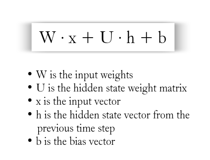
This foundational knowledge is critical if you’re looking into lstm neural network code from scratch or implementing custom architectures.

2. Core Components of the LSTM Cell

Gates and Their Roles

LSTM has three main gates:

• Forget Gate: Determines what information to discard
• Input Gate: Determines what new information to store
• Output Gate: Decides what to output at each time step

Each gate uses a sigmoid activation function to produce values between 0 and 1, allowing the model to make soft decisions.

Cell State and Hidden State

The cell state carries long-term information across time steps, while the hidden state contains short-term information. These are updated through:

This mechanism allows LSTMs to maintain memory over long sequences, addressing a common need in lstm neural network time series forecasting.

3. Activation Functions

Sigmoid and Tanh

The LSTM cell primarily uses two activation functions:

• Sigmoid: Used in gates to squash values between 0 and 1
• Tanh: Used to create candidate values and squash cell state output between -1 and 1

Both functions are differentiable, enabling smooth gradient flow during backpropagation.

---

4. Backpropagation Through Time (BPTT)

Gradient Flow in LSTMs

The training of LSTMs relies on backpropagation through time (BPTT). Unlike feedforward networks, gradients in RNNs flow through time, which can lead to vanishing or exploding gradients. LSTM’s architecture combats this with:

• Constant error carousels in the cell state
• Gate-controlled updates

These innovations enable stable gradient flow, essential for learning long-term dependencies.

---

5. LSTM Mathematical Formulation

Here’s a simplified view of the mathematical operations in a single LSTM cell:

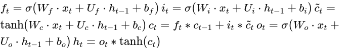
These formulas are the backbone of the lstm neural network architecture.

6. Intuition Behind LSTM Memory

Unlike traditional RNNs, which forget earlier data too quickly, LSTMs retain context effectively. They use the gates to update or forget specific elements of memory.

This is useful for tasks like:

• Language modeling
• Speech recognition
• Machine translation

7. Mathematical Proof of Gradient Stability

Gradient Clipping and Regularization

One of the major strengths of LSTM is its built-in ability to avoid the vanishing gradient problem due to additive interactions in the cell state. However, techniques like gradient clipping and regularization (L2, dropout) can further improve training.

The additive nature of:

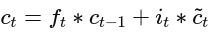
ensures the gradient has a stable path to flow backwards, which is essential for training deep LSTM networks.

8. LSTM vs Traditional RNNs: A Mathematical Perspective

In traditional RNNs:

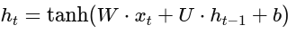
This simplicity leads to issues with long-term learning due to gradient shrinkage. LSTM introduces additional gates and paths to allow better control over information flow.

9. Practical Example of LSTM with Matrix Multiplications

Let’s consider an LSTM implemented in PyTorch:

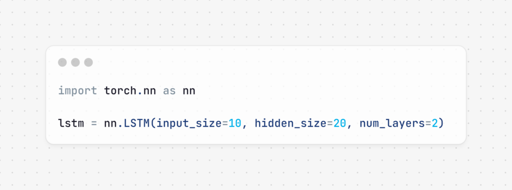
Under the hood, this performs numerous matrix multiplications as described above, which is why knowing the linear algebra behind LSTM helps you debug and improve your models.

10. Next Steps for Learners

To go beyond theory:

• Implement an LSTM from scratch in Python
• Explore variations like GRU and Bi-LSTM
• Apply to real-world tasks like sentiment analysis or financial forecasting

Searches like lstm neural network tutorial for beginners and lstm neural network from scratch are great places to start.

Conclusion

Mastering the mathematical foundations for LSTM neural networks isn’t just for academics—it’s a vital step for any serious machine learning practitioner. By understanding the math behind LSTM, you’ll write better code, train more effective models, and contribute more meaningfully to your team and projects.

This deep dive covered:

• Matrix operations and linear algebra essentials
• Gate mechanisms and memory retention logic
• Gradient flow stability and backpropagation techniques
• High-value subtopics like activation functions and practical examples

Whether you’re optimizing lstm neural network architecture or preparing a lstm neural network tutorial, having this mathematical grounding will always pay off.

FAQs: Mathematical Foundations for LSTM Neural Networks

❓ What is the mathematical basis of LSTM neural networks?

LSTM neural networks are based on matrix operations, sigmoid and tanh activation functions, and a unique gating mechanism that controls the flow of information. They use equations to manage memory cells and hidden states, enabling them to retain information over long sequences.

❓ Why do LSTM networks use sigmoid and tanh functions?

Sigmoid functions are used in the gates to output values between 0 and 1, determining how much information to allow through. Tanh functions are used to squash data within the range of -1 to 1, ensuring stable gradient flow and effective data transformation.

❓ How does LSTM solve the vanishing gradient problem?

LSTMs solve the vanishing gradient problem by using additive updates to the cell state and carefully designed gates. These allow gradients to flow across long sequences without shrinking to near-zero, which commonly happens in traditional RNNs.

❓ What role do matrix operations play in LSTM?

Matrix operations like multiplication and addition are fundamental to how LSTM processes inputs and hidden states at each time step. These operations determine how inputs are combined with learned weights to update memory and output predictions.

❓ Is understanding the math behind LSTM important for implementation?

Yes, having a solid understanding of the mathematical foundations allows you to build LSTM models from scratch, tune them effectively, and debug issues. It also helps in customizing architectures for specific use cases.

❓ Can I learn LSTM neural networks without a math background?

While you can implement LSTM using frameworks like TensorFlow or PyTorch, a basic understanding of linear algebra and calculus will significantly enhance your comprehension and ability to innovate.